|
|
|
 |
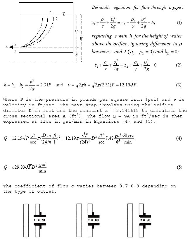
Using the Bernoulli equation and Toricelli's Law, the flow may be expressed as a function of pressure P and outlet diameter D as shown in Figure 2.
Bernoulli was a friend and intellectual rival of legendary physicist
Sir Isaac Newton. J.L. Lagrange (1736-1813) was the first to present the modern form of the equation in his
book Mechanique Analytique published in 1788. Lagrange also listed the assumptions required for the Bernoulli equation to
work. The Bernoulli equation assumes that the fluid and device meet 4 Lagrangian assumptions:
1. The fluid is incompressible
2. The fluid is inviscid
3. The flow is steady
4. The flow is along a streamline
Most liquids meet the incompressible assumption and many gases can even be
treated as incompressible if their density varies only slightly along a streamline from point 1 to point 2.
The steady flow requirement is usually not too hard to achieve for situations typically analyzed by the Bernoulli equation.
Steady flow means that the flow rate (i.e. discharge) does not vary with time. The inviscid fluid requirement implies that the fluid has no viscosity.
All fluids have viscosity although viscous effects are negligible over short distances. The Bernoulli equation is important because it
incorporates the major parameteric components used to describe and analyze the flow of any fluid through pipes or conduits under pressure.
In the Bernoulli equation, fluid flow occurs in response to differences in pressure between two points in a flow stream. Since our experience and intuition often confirms that water tends to flow downhill, the difference in elevation z (ft), between two points in the flow stream is the first component. The fluid column pressure r (lbs/ft2) is the second component. It is divided by the specific weight of the fluid g (62.4 lbs/ft3), to make it consistent with the linear units used in expressing the elevation component. The sum of the two is referred to as the piezometric head or the hydraulic grade line. The third component in the Bernoulli equation is velocity pressure n 2/2g. The sum of the three components, the total head available to the fluid, is called the energy grade line. There is also a head loss component hL which appears on the right side of the equation.
The Hazen-Williams equation for headloss due to friction in pipes flowing full is expressed as:
p is the headloss due to pipe friction (psi/ft).
Q is the pipe flow (gpm).
d is the pipe diameter (in).
C is the Hazen-Williams C-factor in dimensionless units.
The C-factor is a smoothness coefficient for the inner lining of a pipe. Values of C-factor commonly used are listed below:
Pipe Material                 C

Asbestos Cement              140
Brass tube                   130
Cast-Iron tube               100
Concrete tube                110
Copper tube                  130
Corrugated steel tube         60
Galvanized tubing            120
Glass tube                   130
Lead piping                  130
Plastic pipe                 140
PVC pipe                     150
General smooth pipes         140
Steel pipe                   120
Steel riveted pipes          100
Tar coated Cast Iron tube    100
Tin tubing                   130
Wood Stave                   110
The lower the C-factor, the higher the headloss due to pipe friction. The C-factor tends to decrease over time due to pitting and tuberculation on the internal surface of the pipe. The Hazen-Williams equation is the most widely used method for estimating headloss due to friction in pipes.
The Darcy-Weisbach equation includes the effect of fluid turbulence in calculating the headloss due to pipe friction:
where:
hL is the headloss due to pipe friction (ft).
f is the Moody friction factor in dimensionless units.
n is the flow velocity (ft/sec).
L is the length of pipe connecting locations 1 and 2 (ft).
D is the pipe internal diameter (ft).
The Moody f is a function of absolute pipe roughness(e), pipe internal diameter(D) and the Reynolds Number(R). The Reynolds Number is the ratio of inertia forces to viscous forces within the fluid:
where:
D is the internal pipe diameter(ft), V is the flow velocity(ft/sec) and v is the kinematic viscosity(Sq-ft/sec) of water at a given temperature in °F. Fluid flows are laminar for Reynolds Numbers up to 2000. Between 2000 and 4000, the flow is in transition between laminar and turbulent. Beyond a Reynolds Number of 4000, the flow is completely turbulent.
The Moody f friction factor can be graphically determined from the Moody Diagram or by iteratively solving for f in the Colebrook-White Equation:
The Velocity Analyzer utility can be used to quickly and accurately determine the Reynolds Number, Moody f and the Darcy-Weisbach friction based on absolute pipe roughness and kinematic viscosity. The Darcy-Weisbach equation includes the effects of turbulence at high flow velocities. However, it is more complicated to use and yields only a minor improvement in accuracy over the popular Hazen-Williams equation.
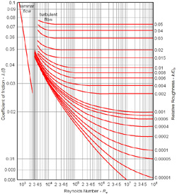 |
The Moody Diagram is a graphical plot of laminar and turbulent flow in pipes as described by the Colebrook-White equation. The one depicted here is a family of curves drawn on logarithmically scaled axes. The right vertical axis is relative roughness(e/D) or the ratio of absolute roughness(Sq-ft/sec) to pipe internal diameter(ft). The Reynolds Number(R) is on the horizontal axis. The Moody f is on the left vertical axis. |
Figure 2: The Hydrant Flow Equation
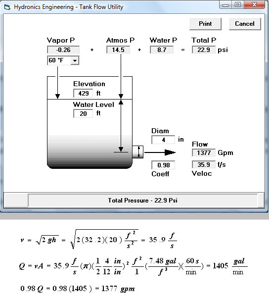
The Tank Flow Utility is used here for estimating the total pressure, flow velocity
and flow from a tank with a 4" diameter spout at a depth of 20' below the water line. As shown in Figure 3,
the water level of 20' in the tank exerts a hydrostatic pressure of 8.7 psi at the spout centerline.
At a temperature of 60°F water has a vapor pressure of 0.26 psi as estimated by the Goff-Gratch Equation.
Since the tank water level is 429' above sea level there is an
atmospheric pressure of 14.5 psi from the overlying column of air. The total pressure at the spout centerline is 14.5 + 8.7 - 0.26 = 22.9 psi.
It should be noted that this is a theoretical estimate of total pressure that must be field verified. The flow of 1378 gallons-per-minute corresponds to a
spout velocity of 35.9 feet-per-second. The 0.98 (98%), for the flow coefficient c, is based on a value of 0.02 (2%) to account for spout entrance and exit losses.
It should again be noted that these are theoretical estimates subject to field verification.
Figure 3: The Tank Flow Utility
A booster pump contains an impeller that is rotated at high speed by a diesel or electric motor. Water is drawn in through
the suction side and into the pump casing where it encounters the spinning impeller. The impeller vanes impart energy to the flow stream and provide a boost to the water pressure
and flow on the discharge side of the pump. The first step in selecting a booster pump is to determine the pressure and flow required by the fire sprinkler system as displayed on the
Booster Pump Dialog. The required pressure and flow are then compared with what is available from the existing water supply system.
A booster pump is necessary if the pressure or flow available from the existing water supply cannot meet the demand required by the fire sprinkler system.
The booster pump must have a rated pressure (psi) and rated flow (gpm) able to meet or exceed the negative difference between what is available and what is required.
The Booster Pump Dialog calculates the rated pressure (psi) and rated flow (gpm) for a typical booster pump per NFPA-20.
It also plots the pump curve and keeps track of important fire pump discharge and suction parameters. The Net Positive Suction Head Available (NPSHa) is determined by adjusting the water pressure at the source for elevation pressure losses, pipe friction losses
and device losses in the piping that connects the water supply source to the suction side of the pump. The next step in booster pump selection involves a basic understanding of pump curves
and the pump parameters NPSHa and Net Positive Suction Head Required (NPSHr).
Figure 4: The Booster Pump Dialog
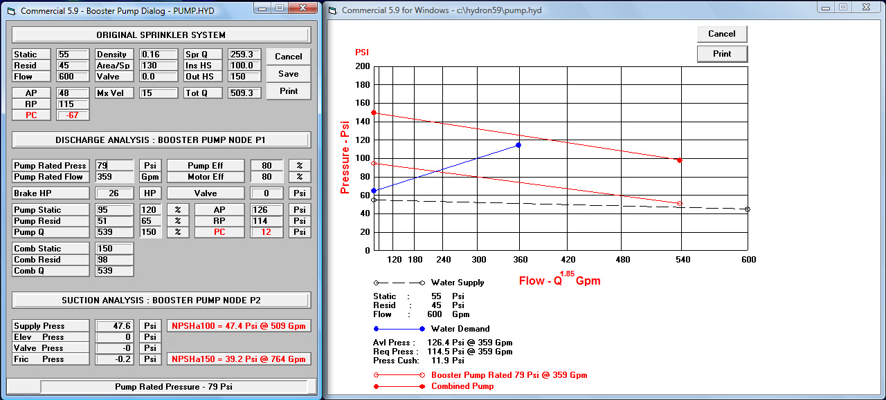
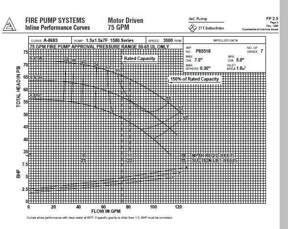
Pump curves are graphical plots of pump pressure (TOTAL HEAD IN PSI on the vertical axis) in relation to pump flow (FLOW IN GPM on the horizontal axis).
The pump churn pressure or shut-off is the point on the pump curve where it intercepts the vertical axis. At churn pressure the pump flow is 0 gpm. The rated pressure and
rated flow are points on the pump curve established by the manufacturer at a given motor speed (rpm), impeller size (inches) and suction pressure (psi).
With the impeller fully submerged, the Net Positive Suction Head Required (NPSHr) is the suction pressure required for the pump to perform as depicted by the pump curve.
Pump curves are reliable indicators of pump performance if the NPSHa measured in the field meets or exceeds the NPSHr.
If the NPSHa drops below the NPSHr, pump performance is degraded and in extreme cases can lead to cavitation and pump failure.
Under field conditions, the available suction pressure or Net Positive Suction Head Available (NPSHa) is affected by pressure losses due to friction, hose demands,
backflow preventers and elevation changes in the piping connecting the water supply source to the suction side of the pump. The lower the NPSHa, the greater the
required pump rated pressure and vice versa. The easiest way to increase NPSHa is to increase the pipe size on the suction side of the pump.
The term K-Factor refers to a set of dimensionless numbers used as coefficients of discharge for
fire sprinklers. They are usually listed along with other fire sprinkler specifications found in manufacturer brochures. But exactly how is a K-Factor determined? The
Bernoulli Equation is a good starting point. Most nozzles and standard deflection type sprinklers yield predictible flows relative to pressure(P)
because the 4 Lagrangian assumptions regarding the flow stream are easily met. However, specially engineered sprinklers have complex internal and
external geometries that may confound the Lagrangian assumptions. The internal vanes in such sprinklers impart a radial velocity component that
creates their characteristically unique spray patterns. As pressure increases, the flow rate may drop because energy losses from turbulence could yield a lower K-Factor.
Turbulent flow makes it virtually impossible to predict friction losses related to changes in pressure. Note that
Q = kÖP = kP0.5 for standard deflection type sprinklers. For specially engineered sprinklers this could
be Q = kP0.44 or Q = kP0.47. In such cases the fire sprinkler must be field tested to obtain Q = kPn
for n<0.5.
A hydraulic simulation model defines and formalizes the linkages between variables that affect the distribution of flow and pressure in a fire sprinkler piping network. It represents a compromise between theoretical complexity and practical reality to the point where the model can be used as a tool for predicting how changes in the design variables will affect the performance and viability of the fire sprinkler system. The model must recognize and accept three major types of data :
Hydraulic calculations are based on the concepts and principles of hydraulics and fluid mechanics expressed in the form of a hydraulic model that incorporates a sequence of pre-defined physical accounting procedures :
A hydraulic calculation may well be the single most important activity associated with designing a fire sprinkler system. The success of a design hinges almost entirely on the extent to which discharging sprinklers can meet the density and flow requirements specified in the design criteria. If the calculations fail, or are in error, the design must be rejected. Hydraulic calculations are usually performed at the bid or preliminary stage of a fire sprinkler project. The results could determine both the physical and economic viability of the sprinkler project. Hydraulic calculations must be done "in house" to ensure flexibility and control over the design process.
In the days when hydraulic calculations were done "by hand", piping geometry was a critical element. Complex loops, grids and compound grid systems were often beyond the capacity of most humans, even those armed with calculators. In fact grid systems had to wait until Professor Hardy Cross ( University of Colorado ) developed his famous technique for iteratively balancing flows in gridded piping systems. The advent of modern high speed digital computers heralded a new age in hydraulic calculations. Mathematical techniques such as finite element, finite difference and Newton-Raphson made it possible to simulate a virtually limitless combination of design parameters. The effect of countless changes in design parameters can be calculated and displayed in a matter of seconds. Developments in computer software such as Microsoft Windows and Apple Macintosh have made it easier to enter and edit data and view the results of hydraulic calculations on the screen or sent to a printer. Hydraulic calculation software have come to symbolize the computerized aspect of a fire sprinkler hydraulic model.